EMO:How EMO models SFT constraints

SFT constraints in SPD

The aim of automatic SFT constraint modelling in EMO is to model the SFT constraints that are generated as part of the dispatch and pricing solution in SPD. These constraints are designed to avoid thermal overloading of a line in the event of the unexpected outage of any other line. SFT constraints appear in the dispatch and pricing optimisation model as linear constraints involving two lines. For example:

 -0.902 × OHK_WRK.1+1.274 × THI_WKM1.1 ≤ 605.79

In this case THI_WKM1.1 is the line being protected from overload and OHK_WRK.1 is the line which may cause overload in THI_WKM1.1 if it has an outage (the contingent line). The general form of the SFT constraint is

Equation 1.

\[ A F_{m} + B F_{c} \leq C \]

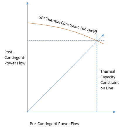
Where \(F_{m}\) is the flow on the protected line and \(F_{c}\) is the flow on the contingent line. The physical nature of the SFT constraint depends on various characteristics of the line being protected, the thermal environment and the mitigating measures available if an outage occurs. The constraint can be expressed as a function of the loading on the line before an outage occurs (pre-contingent) and the loading after an outage occurs (post-contingent). The higher the line is loaded pre-contingency the greater its expected temperature, giving it less capacity to absorb extra power in the event of a contingency.

The physical constraint on the protected line that is modelled with SFT is shown in the diagram 1. This constraint will depend on the thermal environment

Diagram 1. Physical SFT constraint on a single line

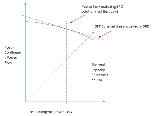
In SPD the constraint above is modelled as a linear constraint which represents a tangent of the physical constraint at the point where the pre-contingent power flow matches the power flow in the solution of SPD. Because the constraint may affect dispatch this is an iterative process, the resulting constraint is shown in diagram 2.

Diagram 2. Physical SFT constraint on a single line

Estimating the constraint curves used by SPD

Up to version 5.2.13 estimates of the constraint curves were based on observing historical constraints (see Estimation From Historical Constraints)

However from version 5.2.13 onwards the thermal characteristics of the circuit are used to calculate the thermal constraint curve. This ensures that previously unconstrained lines may be modelled as effectively as possible. The methods used to define and use the circuit's thermal characteristics are described in EMO:Use of line conductor information in SFT

SFT constraint modelling in EMO

Diagram 1. SFT Protection factor trait in EMO

Among the traits shown for a circuit in EMO is the SFT protection factor, SFT protection factor curvature and SFT threshold (shown here under the columns "SFT PF", "SFT PFQ", "SFT Threshold" respectively). The SFT protection factor and curvature will determine the nature of the SFT constraints generated by EMO. The SFT protection factor is one minus the estimated slope of the thermal constraint curve at the point it passes through the point of maximum thermal capacity. For example if the slope at that point is such that 0.05 MW extra capacity is available for every 1 MW the flow is below the maximum thermal capacity then the SFT protection factor will be 1.05. Setting the SFT protection factor to a high number will tend to relax any constraints on that line. The SFT protection factor curvature is the rate at which this slope changes as the the powerflow is reduced (per 100MW). When making a dispatch with Auto-SFT on EMO will search for lines that may be overloaded by an outage in another line.

The effect of an outage at the contingent line (C) on the power flow on the protected line (M) can be estimated as a proportion of the flow on C being transferred to M.

Equation 4.

\[F'_{m} = F_{m} + B{F}_{m}\]

Where \(F'_{m}\) is the post-contingent flow on the protected line. To ensure the point \(( F_{m}\), \(F'_{m})\) does not lie outside the physical SFT constraint in Diagram 1 above, a linear constraint is added to the dispatch model as follows

Equation 5.

\[AF_{m} + BF_{c} \leq A \underline{C}\]

Where A is equal to the slope of the tangent line to the thermal constraint curve and C is the y-intersect of this line. Once the exposed lines are identified and the related constraints are added to the model the dispatch is reiterated. Eventually all relevant SFT constraints should be found and applied.