EMO:How EMO models SFT constraints
SFT constraints in SPD
The aim of automatic SFT constraint modelling in EMO is to model the SFT constraints that are generated as part of the dispatch and pricing solution in SPD. These constraints are designed to avoid thermal overloading of a line in the event of the unexpected outage of any other line. SFT constraints appear in the dispatch and pricing optimisation model as linear constraints involving two lines. For example:
-0.902 × OHK_WRK.1+1.274 × THI_WKM1.1 ≤ 605.79
In this case THI_WKM1.1 is the line being protected from overload and OHK_WRK.1 is the line which may cause overload in THI_WKM1.1 if it has an outage (the contingent line). The general form of the SFT constraint is
| Equation 1. | \[ A F_{m} + B F_{c} \leq C \] |
Where \(F_{m}\) is the flow on the protected line and \(F_{c}\) is the flow on the contingent line. The physical nature of the SFT constraint depends on various characteristics of the line being protected, the thermal environment and the mitigating measures available if an outage occurs. The constraint can be expressed as a function of the loading on the line before an outage occurs (pre-contingent) and the loading after an outage occurs (post-contingent). The higher the line is loaded pre-contingency the greater its expected temperature, giving it less capacity to absorb extra power in the event of a contingency.
The physical constraint on the protected line that is modelled with SFT is shown in the diagram 1. This constraint will depend on the thermal environment

In SPD the constraint above is modelled as a linear constraint which represents a tangent of the physical constraint at the point where the pre-contingent power flow matches the power flow in the solution of SPD. Because the constraint may affect dispatch this is an iterative process, the resulting constraint is shown in diagram 2.

Estimating the constraint curves used by SPD
The power flows used in this relationship are from an AC power flow model, which is constructed using the SPD solution in conjunction with reactive power modelling and a detailed model of the transmission grid componentry. The full information for creating this AC model is not available to us, so there is an inevitable degree of approximation in estimating SFT constraints from our point of view. To model this constraint in EMO we also need to estimate the nature of the pre-post power flow constraint for each line. We do not currently have access to the definitions of these functions, but we are informed that they are quadratic functions and they will pass through the point \(( \underline{C}, \underline{C} )\) where \(\underline{C}\) is the thermal capacity of the line, which is a value we do have access to. Given that the constraint is a quadratic function and we know one point on the function there are two degrees of freedom left to estimate. Here we look at estimating \(\beta\), the slope of the curve at \(( \underline{C}, \underline{C} )\), and \(\alpha\), the rate of change in that slope with respect to \(F_{m}\).
The slope of the tangent of this curve at \(F_{m}\) is given explicitly in the resulting constraint equation in SPD, being negative the value A in Equation 1. We have the arc flows \(F_{m}\) from the SPD solution so, given enough instances of an SFT equation for a particular protected line, we might be able to estimate its pre-post constraint curve. We are informed that the thermal environment used for each curve is purely dependent on the Summer/Shoulder/Winter designation of the trading period so we can make a sample of all the constraints that fall into each category.
To estimate the curve then we can try to find the linear relationship between the slope and the pre-contingent flow. Given all equations associated with a particular combination of SFT constraint and thermal environment, we are looking for values of \(\alpha\) and \(\beta\) which have the following relationships. If a good fit for these values can be found the quadratic curve can be estimated.
| Equation 2. | \[A \simeq \alpha \big(\underline{C} - \underline{F}_{m} \big)+\beta\] |
| Equation 3. | \[C \simeq \underline{C} + \frac{ \alpha }{2} \big(\underline{C} - \underline{F}_{m} \big)^{2}\] |
However there appears to be no significant and reliable correlation between the tangent slope of the SFT constraints (A in Equation 1) and the power flows in the solution in the data we have analysed to date. What correlation there is appears to be overshadowed by the variability in the limit, which is sometimes seen to fall below the \(\big( \underline{C}, \underline{C} \big)\) point, probably due to the effects of reactive power flows. For these reasons the best fit is currently calculated by setting \(\alpha\) to 0 and \(\beta\) to the average slope A.
These values are delivered to EMarketOffer using the AverageLineProtectionFactors<date>.csv file in the <EMO Data Dir>/Inputs/Grid/SFT directory. Lines for which we have no data have these values set to 0 and 1.04, which is the average protection value for lines which are not under enhanced protection schemes.
The \(\alpha\) and \(\beta\) values can then be used to generate slopes and constraint limits for all values of \(F_{m}\), they are referred to here as the ‘SFT constraint curvature’ and the ‘SFT protection factor’ respectively. Only the latter currently appears in EMO as an input value against each line, the variation value being set to zero.
Some examples of constraint variation are shown in the figures below:
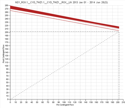
Figure 1: Summer SFT constraints on the NSY_ROX.1 line (contingent line CYD_TWZ1.1)
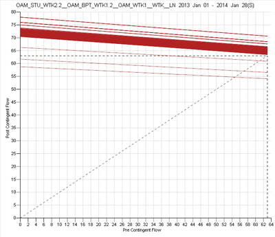
Figure 2: Summer SFT constraints on the OAM_STU_WTK2.2 line (contingent line OAM_BPT_WTK1.2)
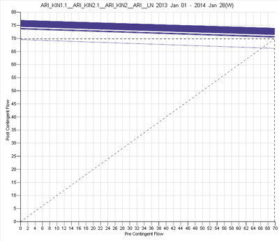
Figure 3: Winter SFT constraints on the ARI_KIN1.1 line (contingent line ARI_KIN2.1)
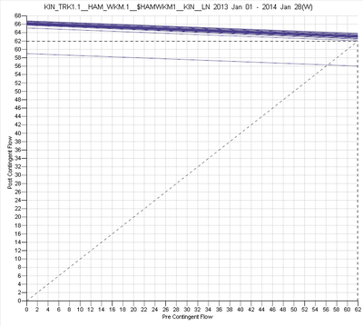
Figure 3: Winter SFT constraints on the KIN_TRK1.1 line (contingent line HAM_WKM.1)


SFT constraint modelling in EMO

Among the traits shown for a circuit in EMO is the SFT protection factor (shown here under the column SFT). There is no trait currently for the SF constraint curvature. The SFT protection factor will determine the nature of the SFT constraints generated by EMO. Setting the SFT protection factor to a high number will tend to relax any constraints on that line. When making a dispatch with Auto SFT on EMO will search for lines that may be overloaded by an outage in another line. The effect of an outage at the contingent line (C) on the power flow on the protected line (M) can be estimated as a proportion of the flow on C being transferred to M.
| Equation 4. | \[F'_{m} = F_{m} + B{F}_{m}\] |
Where \(F'_{m}\) is the post-contingent flow on the protected line. To ensure the point \(( F_{m}\), \(F'_{m})\) does not lie outside the physical SFT constraint in Diagram 1 a linear constraint is added to the dispatch model as follows
| Equation 5. | \[AF_{m} + BF_{c} \leq A \underline{C}\] |
Where A is equal to the protection factor on the protected line. Once the exposed lines are identified and the related constraints are added to the model the dispatch is reiterated. Eventually all relevant SFT constraints should be found and applied.